In my last Innovation Papers post, I approached the subject of Deep Learning and introduced the concept of Neural Networks, which I had began to understand through Andrew Ng’s Coursera course on the matter. We got as far as introducing these computing constructions called neural networks (due to their “shape” being similar to neuron cells), which are capable of identifying patterns in the information we input, allowing them to distinguish between different sets of data (it is or it is not the picture of a cat). That is great, and certainly most useful. However, it is not my objective to speak about the possible applications of Deep Learning using neural networks, but instead to try to explain, in simple terms, how they are able to do what they do, as well as how surprising it was for me to see its simplicity.

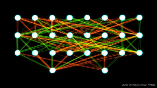
As I explained in my previous post, a neural network is composed of layers of “neurons”. Each neuron of a layer receives all the inputs, performs some calculations, and outputs a value. These outputs become the inputs of the next layer, and so on, until the final output layer. So what are these calculations? Normally, or at least as far as my knowledge of the matter goes, the calculation in each neuron is composed of two steps. A linear calculation and a non-linear one; don’t worry, I will try not getting very technical.

The first step consists on applying a linear function of the type mx+b to the input. Both m and x are vectors: (x0, x1, x2…xi…) and (m0, m1, m2, … mi…), which for the sake of our discussion, just means that they are sets of numbers. In this case, x is the set of values we input to the neuron, and m a set of constants we multiply each of the input values by. The result of the calculation would then be m0.x0+m1.x1+…+mi.xi+…+b, which would give us just a single number. The values of m and b are specific to each neuron, while the values of x correspond to the variable data we input to the neuron. From this, you only need to retain that we multiply each value of the input by a different number and add them all together also with another number b; simple multiplication and addition, nothing fancy or complicated.

In the second step, each neuron applies an “activation function”, which is a non-linear function probably more difficult to understand (ReLU, sigmoid, …), but you actually don’t need to. To simplify, for instance, if we use a sigmoid function (https://en.wikipedia.org/wiki/Sigmoid_function), it just transforms the input into a number between 0 and 1.

All the outputs of the neurons of the first layer, become the inputs of each neuron of the second layer and so on, until we reach the final layer. This final, or output layer, would have a single neuron in our basic binary neural network, that will output a number between 0 and 1. We would assume the final answer to be “no” if this value is between 0 and 0.5 and “yes” if it is between 0.5 and 1.

If I have lost you, let me use the cat picture as an example. A digital picture is composed of pixels and, to simplify, let’s assume it is a greyscale picture (no colour). Each pixel would have a value, for instance between 0 (black) and 255 (white) which indicates the shade of grey of the pixel. With this information we would build a vector (a set) with the value of each and every pixel in the picture. This set would become x, the input to each and every neuron of the first layer of the neural network. Each neuron would do their calculations and produce an output which would be different for each of them (m‘s and b‘s are different for each neuron). All these values, in turn, become the input for each neuron in the second layer and so on until the end, where we would receive a “yes” if the initial input was the picture of a cat or a “no” if it wasn’t…

Magic? No, not really, but the trick is of course in the values of the parameters m and b of each neuron. And how do we know which values we should give to each neuron to do what we want it to do? Well, the beauty of it is that we don’t. What we do is “train” the network. To put it in simple terms, we just initialise the parameters of the neurons with random values and we make the network operate on a large number of input datasets (pictures in our example) where we know the correct answer from. For instance, a set of “cat” or “non-cat” pictures, so we know what the correct answer should be for each picture. Then, we compare the actual output produced by the network for each picture to the correct answer it should have given in each case. Let’s say that we count one for each mistake and zero for each correct result; we will call this the “Cost Function”. Our objective would then be to train the network, that is, to modify the parameters m and b of each neuron, so the result of the Cost Function is as closer to zero (no mistakes) as possible.

But how can we “teach” the network to learn from its mistakes? Should we try using other random values for the parameters and see how the network performs? Well, with enough time and computing power, we could, but no one knows how long it would take to find the right set of values. What is actually done in Deep Learning algorithms is to use “backward propagation”, and I am afraid this is more mathematically complex to explain as it involves derivatives, but let me try to give a simple explanation. The idea is based on the concept of “Gradient Descent”.

Imagine you are lost in a mountain and want to climb down, but there is a thick fog and you cannot see much further than your own feet. What you can do, is see which is the direction around you which has the steepest slope down, and take a step in that direction. After that, you look again and take another step in the steepest direction down from that point, and so on until you reach the bottom. Of course this is a mathematical construct that only works if there are no “local minima”, that is, your mountain is a single peak (if you are inside the crater of a volcano, this rule will bring into the crater, not down the mountain). We apply this Gradient Descent concept to the Cost function (defining in a way that it has a single minimum), moving backwards through the layers of the network modifying slightly the value of the parameters (m and b) of each neuron in the direction of the steepest slope (this is done using derivatives, which actually are the representation of the “slope” of the function). In this way, we calculate new values for the parameters, which we use to run again the training dataset through the network, hopefully, getting a better (lower) value for the Cost function (closer to no mistakes). If we repeat the process through a number of forward and backwards iterations, normally the network will converge and reach an optimum value of the parameters. Once our network is trained, we can use it with “unknown” pictures to determine if it is or it isn’t the picture of a cat, or whatever objective we use the network for.

Magic, I ask again? No, but it is certainly a neat trick. But why does it work? How can something so simple as a few simple operations and with random initial values work so well? Is pattern recognition really learning? I am afraid the post is too long already to go into this, but I leave you with a link to an explanation of why deep learning works (https://www.quantamagazine.org/new-theory-cracks-open-the-black-box-of-deep-learning-20170921), as well as another one to a tutorial where you can experiment with neural networks (www.technologyreview.com/the-download/609085/this-fun-ai-tutorial-highlights-the-limits-of-deep-learning). I will be happy to discuss with any of you in the comments or elsewhere your thoughts about it, of course being far from an expert myself.

I hope this small contribution has been able to help you understand a little better the subject of Deep Learning and, hopefully, stirred your curiosity and desire to learn more about it. Which brings me to another question: How do we learn?